Fraud attacks are getting sophisticated. Scripted bot registrations, low-value card testing, and cross-border stolen card usage are increasingly common, and the window between attack start and financial damage is shrinking. Sift already flags individual fraudulent transactions in sub-seconds. The harder problem is catching the pattern behind a coordinated attack, as it can run for hours, before anyone notices. The consequences are concrete: a BIN attack can run for hours before an analyst notices the decline rate spike. A registration bot surge can create thousands of fake accounts before anyone spots the velocity anomaly. A card testing campaign using low-value transactions can fly under the radar entirely because existing tools don’t flag successful low-value transactions as suspicious. Each of these scenarios represents real financial loss and reputational damage for the customer.
The Attack Detection Agent is our real time layer that evaluates every scored event as it happens and detects anomalies for relevant traffic patterns.
The Challenge
Sift scores thousands of events per second (orders, transactions, chargebacks, account creations) across every customer we protect. Every scored event is published to the Kafka topic, carrying the original event details (type, user, card BIN, amount, status). That stream is a good data source for real-time detection, if you can read it fast enough, and if you can tell, at any moment, what “normal” looks like for the customer who just sent it.
That second part is hard. Every customer has different traffic, different hours of activity, different set of card BINs, different chargeback rate. A spike that’s alarming for one customer is normal traffic for another. So the system needs to learn a seasonal baseline per customer, per time period, per day of week, and compare live traffic against that customer’s normal.
For this first phase, we scoped in four attack patterns worth watching for in real time:
- BIN attacks (card testing): a burst of distinct card numbers or users per a single BIN, often with a high decline rate, as an attacker probes for live cards.
- Low-value transaction surges: a customer-wide spike in tiny transactions, a signature of distributed card testing.
- Registration velocity surges: an abnormal burst of new account creation, often the first stage of an account-takeover campaign.
- Chargeback / fraud-rate spikes: a rise in confirmed fraud that’s slower to surface but still worth flagging automatically.
Detect these patterns within minutes wherever possible and keep every detection explainable. A customer-facing alert has to say exactly which metric crossed which threshold and detection must happen without slowing down the existing scoring path.
Architecture
We implemented a three-stage pipeline:
- Data Ingestion streams the live scoring events into a database.
- Sensor layer trains a per-customer seasonal forecast and flags deviations from it.
- Alerter service turns those signals into deduplicated, actionable notifications delivered exactly once.
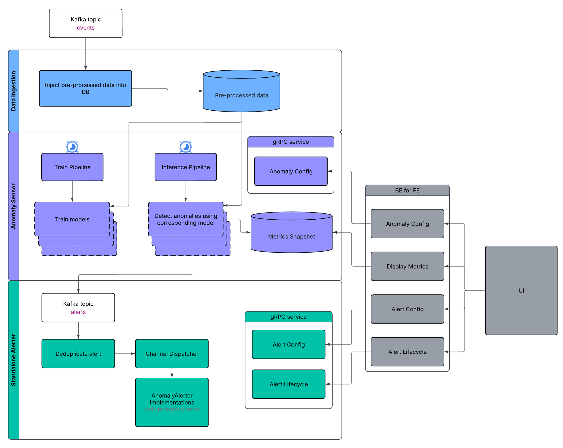
The three-stage pipeline: Data Ingestion, Sensor, and Alerter each run and scale independently.
The hardest part was the Anomaly Sensor, since different anomaly types involve different statistical patterns, so no single detection approach works well across all of them. We designed for flexibility so each anomaly type can use a sensor implementation that gives the best accuracy. Adding a new anomaly type, requires a new sensor and a notification template for the Alerter. Ingestion, Sensor, and Alerter are decoupled, so each one can change independently.
Data Ingestion
The ingestion uses a Kafka connector that reads every scored event and streams into a single table. The data is filtered at write time to persist only required event types anomaly detection needs (orders, transactions, chargebacks). The table is keyed by event time and customer and carries a small set of fields relevant to anomaly detection.
Training and inference happen downstream against this one table.
Anomaly Sensor
This is where anomaly detection happens. It consists of these parts: Train Pipeline, Inference Pipeline, Anomaly Config storage, Metric Snapshot storage.
Train Pipeline
An Airflow-orchestrated Train Pipeline builds a seasonal forecasting model directly against pre-processed data. Full models retrain happens daily to provide precise forecasts based on recent changes in traffic patterns. Train Pipeline builds individual models per-customer, per-anomaly type. Train models are stored as temporal tables in the database and reused by Inference Pipeline.
Inference Pipeline
Inference Pipeline runs frequently to provide near-real time anomaly detection. It compares the latest time period’s observed metric against the model’s forecast. Inference Pipeline returns a model forecast, an expected normal range, its corresponding percentile for the given prediction interval and the standard deviation (Z-score). Basically it looks at whether “this metric is outside its expected range for this period of time”. The Inference Pipeline output is stored as Metric Snapshot to show historical trends for a specific metric on UI.
Previously detected anomalies are explicitly excluded from the training data so that they do not affect normal traffic trends.
BIN attacks are watched with two independent metrics, event count per BIN (burst of card-testing volume) and distinct user id cardinality per BIN. We use HyperLogLog to keep it cheap at scale (catching an attacker spreading the same BIN across many stolen identities). Each metric is modeled and evaluated independently and can fire its own alert. A BIN with an unexpected number of raw transactions and a BIN with an unexpected number of distinct users, are two separate anomalies.
A low-value surge anomaly is an unexpected increase in small value transactions. Each customer has a unique value for what “low-value transaction” means. For example, it could be $2 for one customer and $20 for another.
A registration surge anomaly is an unexpected volume of new accounts created.
A chargeback spike is a chargeback rate outside its usual range for that customer.
Here’s roughly what that looks like for a BIN attack. It is a sudden spike in distinct users on one card BIN, outside the range the model expects for that time period:
[Forecast chart: observed distinct users on a card BIN spiking sharply above the model’s forecasted range, with the spike flagged as an anomaly]
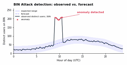
Inference Pipeline evaluates all anomaly models across all customers in minutes.
Anomaly Config
Every anomaly type can be configured by the customer. A customer can select the sensitivity for an anomaly. Customers can set a minimum-volume guard so low volume customers don’t get meaningless alerts. Some customers require fixed thresholds, for example to alert when “number of new account registration exceeds specific number”. To cover these we support fixed thresholds.
Bucketing BINs by Popularity
The walkthrough above glosses over one tricky problem specific to BIN attacks: what’s the “series” you’re actually forecasting? For a registration surge or a chargeback spike, there’s one series per customer, one seasonal baseline to learn, one metric to evaluate. A BIN attack is different. It shows up on individual card BINs, and a single active customer can have tens of thousands of distinct BINs moving through it in a given period of time. Training a dedicated model as one series per (customer, BIN) pair means fitting and continuously retraining tens of thousands of independent seasonal models per customer. Most of the BINs see a handful of transactions a day. It is not enough to build a meaningful seasonal baseline. That’s slow to train, expensive to keep fresh on a rolling basis, and mostly wasted effort. A model trained on five data points a day isn’t telling you anything a fixed minimum-volume guard couldn’t already tell you for free.
The solution we shipped: don’t train individual models for every BIN. Bucket BINs by how much traffic they actually see, and train one shared model per bucket instead. For each customer and every time period, we rank card BINs by volume and assign each one to a popularity bucket based on where it falls in that customer’s own distribution:
CASE

  WHEN event_count <= PERCENTILE_CONT(0.75) WITHIN GROUP (ORDER BY event_count)

    OVER (PARTITION BY customer_id) THEN 'low'

  WHEN event_count <= PERCENTILE_CONT(0.95) WITHIN GROUP (ORDER BY event_count)

    OVER (PARTITION BY customer_id) THEN 'medium'

  WHEN event_count <= PERCENTILE_CONT(0.99) WITHIN GROUP (ORDER BY event_count)

    OVER (PARTITION BY customer_id) THEN 'high'

  ELSE bin  -- top 1% of BINs get their own series

END AS bin_popularity_bucket
Everything below the 99th percentile collapses into three shared series per customer (low, medium, high), instead of one series per BIN. The median of the bucket metric is used as the value to train on.
SELECT

  customer_id || ':' || bin_popularity_bucket AS series,

  time_bucket,

  MEDIAN(event_count) AS median_event_count

FROM bucketed_data

GROUP BY customer_id, bin_popularity_bucket, time_bucket
That collapses what could be thousands of per-BIN series for a large customer down to three main buckets and a bunch of the top BINs. The top 1% of BINs by volume are the ones with enough history and enough transaction weight to matter on their own. They skip the bucketing entirely and keep an individual series, so we don’t lose resolution on the most popular BINs a customer would care most about. In practice, the Train Pipeline across all of our bucketed BIN-attack models now finishes in around 15 minutes, down from roughly an hour before.
Sharing a training series doesn’t mean sharing an anomaly outcome, though. At inference time, every individual BIN is associated with its current popularity bucket based on historical metric trend. The specific BIN’s current-period metric value (not bucket-wide aggregate) gets compared against the forecast and expected range produced by its bucket’s shared model. Inference Pipeline flags a BIN when that BIN’s own value falls outside the range its bucket expects. Two BINs sitting in the same “medium” bucket in the same time period can land on different outcomes depending on their own traffic. What’s shared across BINs in a bucket is the seasonal baseline, not the anomaly decision itself. Each flagged BIN still gets its own row in Metric Snapshot storage, named individually under (customer, BIN) series.
Want to Build This With Us?
This project uses a bunch of different tools: Kafka, Airflow orchestration, Spanner, a standalone gRPC service, and a fair amount of real distributed-systems thinking about deduplication and alert state. If the kind of problems in this post, like real-time systems, explainable applied ML, fighting fraud, sound like a problem you want to work on, we’re hiring. Come build the next phase with us – open reqs
Authors: Artem Dvornichenko, Dima Mostovyi, Eduard Chumak and Oleksandr Kochkodan
Edited & Reviewed: Jason Fama and Ankush Walhekar